Internal convention

+ View the NASA Portal

Search JPL

Internal convention

Starting with version 1.20 (released in Feb 2003),HEALPix uses the same conventions as CMBFAST for the sign and normalization of the polarization power spectra, as exposed below (adapted from [Zaldarriaga (1998)]). How this relates to what was used in previous releases is exposed in A.3.2.

The CMB radiation field is described by a $2\, \times \, 2$ intensity tensor I_ij [Chandrasekhar (1960)]. The Stokes parameters Q and U are defined as Q=(I₁₁-I₂₂)/4 and U=I₁₂/2, while the temperature anisotropy is given by T=(I₁₁+I₂₂)/4. The fourth Stokes parameter V that describes circular polarization is not necessary in standard cosmological models because it cannot be generated through the process of Thomson scattering. While the temperature is a scalar quantity Q and U are not. They depend on the direction of observation ${\bf n}$ and on the two axis $({\bf {e}_{1}}, {\bf {e}_{2}})$ perpendicular to ${\bf n}$ used to define them. If for a given ${\bf n}$ the axes $({\bf {e}_{1}}, {\bf {e}_{2}})$ are rotated by an angle $\psi$ such that ${{\bf {e}_{1}}}^{\prime}=\cos \psi \ {{\bf {e}_{1}}}+\sin\psi \ {{\bf {e}_{2}}}$ and ${{\bf {e}_{2}}}^{\prime}=-\sin \psi \ {{\bf {e}_{1}}}+\cos\psi \ {{\bf {e}_{2}}}$ the Stokes parameters change as

$\displaystyle Q^{\prime}$	$\textstyle \myequal$	$\displaystyle \cos 2\psi \ Q + \sin 2\psi \ U$
$\displaystyle U^{\prime}$	$\textstyle \myequal$	$\displaystyle -\sin 2\psi \ Q + \cos 2\psi \ U$	(5)

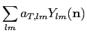
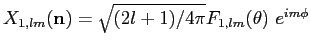
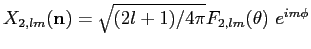
To analyze the CMB temperature on the sky, it is natural to expand it in spherical harmonics. These are not appropriate for polarization, because the two combinations $Q\pm iU$ are quantities of spin $\pm 2$ [Goldberg (1967)]. They should be expanded in spin-weighted harmonics $\, _{\pm2}Y_l^m$ [Zaldarriaga & Seljak (1997)], [Seljak & Zaldarriaga (1997)],

$\displaystyle T({\bf n})$	$\textstyle \myequal$	$\displaystyle \sum_{lm} a_{T,lm} Y_{lm}({\bf n})$
$\displaystyle (Q+iU)({\bf n})$	$\textstyle \myequal$	$\displaystyle \sum_{lm} a_{2,lm}\;_2Y_{lm}({\bf n})$
$\displaystyle (Q-iU)({\bf n})$	$\textstyle \myequal$	$\displaystyle \sum_{lm} a_{-2,lm}\;_{-2}Y_{lm}({\bf n}).$	(6)

To perform this expansion, Q and U in equation (6) are measured relative to $({\bf {e}_{1}}, {\bf {e}_{2}})=({\bf {e}_\theta}, {\bf {e}_\phi})$ , the unit vectors of the spherical coordinate system. Where ${\bf {e}_\theta}$ is tangent to the local meridian and directed from North to South, and ${\bf {e}_\phi}$ is tangent to the local parallel, and directed from West to East. The coefficients $_{\pm 2}a_{lm}$ are observable on the sky and their power spectra can be predicted for different cosmological models. Instead of $_{\pm 2}a_{lm}$ it is convenient to use their linear combinations

a_E,lm	$\textstyle \myequal$	-(a_2,lm+a_-2,lm)/2
a_B,lm	$\textstyle \myequal$	-(a_2,lm-a_-2,lm)/2i,	(7)

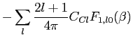
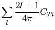
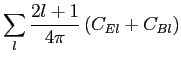
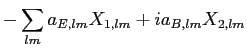
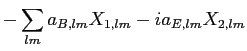
which transform differently under parity. Four power spectra are needed to characterize fluctuations in a gaussian theory, the autocorrelation between T, E and B and the cross correlation of E and T. Because of parity considerations the cross-correlations between B and the other quantities vanish and one is left with

$\displaystyle \langle a_{X,lm}^{*} a_{X,lm^\prime}\rangle$

$\textstyle \myequal$

$\displaystyle \delta_{m,m^\prime}C_{Xl} \quad \langle a_{T,lm}^{*}a_{E,lm}\rangle=\delta_{m,m^\prime}C_{Cl},$

(8)

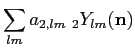
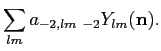
where X stands for T, E or B, $\langle\cdots \rangle$ means ensemble average and $\delta_{i,j}$ is the Kronecker delta.

We can rewrite equation (6) as

$\displaystyle T({\bf n})$	$\textstyle \myequal$	$\displaystyle \sum_{lm} a_{T,lm} Y_{lm}({\bf n})$
$\displaystyle Q({\bf n})$	$\textstyle \myequal$	$\displaystyle -\sum_{lm} a_{E,lm} X_{1,lm} +i a_{B,lm}X_{2,lm}$
$\displaystyle U({\bf n})$	$\textstyle \myequal$	$\displaystyle -\sum_{lm} a_{B,lm} X_{1,lm}-i a_{E,lm} X_{2,lm}$	(9)

where we have introduced $X_{1,lm}({\bf n})=(\;_2Y_{lm}+\;_{-2}Y_{lm})/2$ and $X_{2,lm}({\bf n})=(\;_2Y_{lm}-\;_{-2}Y_{lm})/ 2$ . They satisfy Y^*_lm = (-1)^m Y_l-m, X^*_1,lm=(-1)^m X_1,l-m and X^*_2,lm=(-1)^m+1X_2,l-m which together with a_T,lm=(-1)^m a_T,l-m^*, a_E,lm=(-1)^m a_E,l-m^* and a_B,lm=(-1)^m a_B,l-m^* make T, Q and U real.

In fact $X_{1,lm}({\bf n})$ and $X_{2,lm}({\bf n})$ have the form, ${X_{1,lm}({\bf n})=\sqrt{(2l+1) / 4\pi} F_{1,lm}(\theta)\ e^{im\phi}}$ and ${X_{2,lm}({\bf n})=\sqrt{(2l+1) / 4\pi} F_{2,lm}(\theta)\ e^{im\phi}}$ , ${F_{(1,2),lm}(\theta)}$ can be calculated in terms of Legendre polynomials [Kamionkowski et al (1997)]

$\displaystyle F_{1,lm}(\theta)$	$\textstyle \myequal$	$\displaystyle N_{lm} \left[ -\left({l-m^2 \over \sin^2\theta} +{1 \over 2}l(l-... ... \theta) +(l+m) {\cos \theta \over \sin^2 \theta} P_{l-1}^m(\cos\theta)\right]$
$\displaystyle F_{2,lm}(\theta)$	$\textstyle \myequal$	$\displaystyle N_{lm}{m \over \sin^2 \theta} [ -(l-1)\cos \theta P_l^m(\cos \theta)+(l+m) P_{l-1}^m(\cos\theta)],$	(10)

where

$\displaystyle N_{lm}(\theta)$

$\textstyle \myequal$

$\displaystyle 2 \sqrt{(l-2)!(l-m)! \over (l+2)!(l+m)!}.$

(11)

Note that $F_{2,lm}(\theta)=0$ if m=0, as it must to make the Stokes parameters real.

The correlation functions between 2 points on the sky (noted 1 and 2) separated by an angle $\beta$ can be calculated using equations (8) and (9). However, as pointed out in [Kamionkowski et al (1997)], the natural coordinate system to express the correlations is one in which ${\bf {e}_{1}}$ vectors at each point are tangent to the great circle connecting these 2 points, with the ${\bf {e}_{2}}$ vectors being perpendicular to the ${\bf {e}_{1}}$ vectors. With this choice of reference frames, and using the addition theorem for the spin harmonics [Hu & White (1997)],

$\displaystyle \sum_m \;_{s_1} Y_{lm}^*({\bf n}_1) \;_{s_2} Y_{lm}({\bf n}_2)$

$\textstyle \myequal$

$\displaystyle \sqrt{2l+1 \over 4 \pi} \;_{s_2} Y_{l-s_1}(\beta,\psi_1)e^{-is_2\psi_2}$

(12)

we have [Kamionkowski et al (1997)]

$\displaystyle \langle T_1T_2 \rangle$	$\textstyle \myequal$	$\displaystyle \sum_l {2l+1 \over 4 \pi} C_{Tl} P_l(\cos \beta)$
$\displaystyle \langle Q_{r}(1)Q_{r}(2) \rangle$	$\textstyle \myequal$	$\displaystyle \sum_l {2l+1 \over 4 \pi} [C_{El} F_{1,l2}(\beta)-C_{Bl} F_{2,l2}(\beta)]$
$\displaystyle \langle U_{r}(1)U_{r}(2) \rangle$	$\textstyle \myequal$	$\displaystyle \sum_l {2l+1 \over 4 \pi} [C_{Bl} F_{1,l2}(\beta)-C_{El} F_{2,l2}(\beta) ]$
$\displaystyle \langle T(1)Q_{r}(2) \rangle$	$\textstyle \myequal$	$\displaystyle - \sum_l {2l+1 \over 4 \pi} C_{Cl} F_{1,l0}(\beta)$
$\displaystyle \langle T(1)U_{r}(2) \rangle$	$\textstyle \myequal$	0.	(13)

The subscript r here indicate that the Stokes parameters are measured in this particular coordinate system. We can use the transformation laws in equation (5) to write (Q,U) in terms of (Q_r,U_r).

The definitions above imply that the variances of the temperature and polarization are related to the power spectra by

$\displaystyle \langle TT \rangle$	$\textstyle \myequal$	$\displaystyle \sum_l {2l+1 \over 4 \pi} C_{Tl}$
$\displaystyle \langle QQ \rangle + \langle UU\rangle$	$\textstyle \myequal$	$\displaystyle \sum_l {2l+1 \over 4 \pi} \left(C_{El} +C_{Bl}\right)$
$\displaystyle \langle TQ\rangle = \langle TU\rangle$	$\textstyle \myequal$	0.	(14)

It is also worth noting that with these conventions, the cross power C_Cl for scalar perturbations must be positive at low l, in order to produce at large scales a radial pattern of polarization around cold temperature spots (and a tangential pattern around hot spots) as it is expected from scalar perturbations [Crittenden et al (1995)].

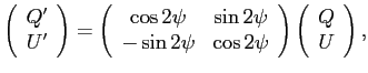
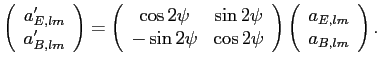
Note that Eq. (9) implies that, if the Stokes parameters are rotated everywhere via

$\displaystyle \left(\begin{array}{c} Q'\\ U' \end{array}\right) = \left(\be... ...array} \right) \left(\begin{array}{c} Q\\ U \end{array} \right),%\nonumber$

(15)

then the polarized a_lm coefficients are submittted to the same rotation

$\displaystyle \left(\begin{array}{c} a_{E,lm}'\\ a_{B,lm}' \end{array}\right... ... \left(\begin{array}{c} a_{E,lm}\\ a_{B,lm} \end{array} \right).%\nonumber$

(16)

Finally, with these conventions, a polarization with (Q>0,U=0) will be along the North-South axis, and (Q=0,U>0) will be along a North-West to South-East axis (see Fig. 5)

Eric Hivon 2010-06-18

Contact:

Site Manager:
Webmaster:
CL 03-2650